
 mufasa-fusion
Railway security#
Field-tested
Use cases: Trespassing Sabotage Vandalism
Detection along railway corridors, by day and at night.
At a glance#
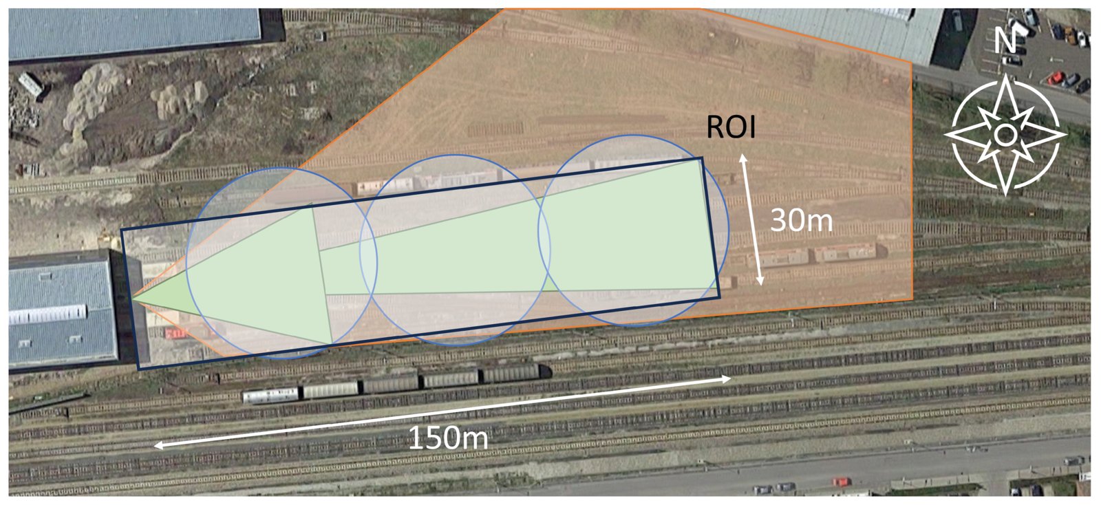
Sensor setup of the trial: thermal cameras (green), acoustic sensors (blue), radar (orange) and the 150 m × 30 m region of interest (black). From Hubner et al., Sensors 2024, CC BY 4.0.#
Objects of interest |
Persons, objects placed on the track, vandalism such as breaking glass or spray-can use |
Sensors |
Thermal camera, radar, acoustic sensors |
Platform |
Fixed: stationary sensors monitoring a defined track section |
Setting |
Controlled real-world environment, day and night |
How MuFASA was used |
Iterative parameter refinement within one fixed architecture |
How MuFASA was used#
One graph, many experiments. Temporal decay rates and detection thresholds were varied systematically to characterise the behaviour under day and night conditions: change a parameter, re-run, inspect the output.
From recorded to live. Data was recorded and analysed offline first. The same graph then went live by exchanging the file input nodes for streaming input nodes, connected to the sensors via ROS2.
The Fusion Graph#
One of the sensor combinations of the trial: each sensor accumulates its detections into a probability map, the three maps are fused, and a threshold turns the fused map into alarms.
from mufasa import BoundingBox, Graph
from mufasa.io.inputs import GeoJsonInput
from mufasa.io.outputs import GeoJsonOutput
from mufasa.nodes import POM, BayesianFusion, Threshold

# Input nodes: one per sensor
thermal = GeoJsonInput("thermal.geojson")
radar = GeoJsonInput("radar.geojson")
acoustic = GeoJsonInput("acoustic.geojson")

# Processing nodes: each sensor with its own decay and baseline confidence
fused = BayesianFusion()(
    POM(decay_s=3, prior=0.7)(thermal),
    POM(decay_s=5, prior=0.7)(radar),
    POM(decay_s=10, prior=0.55)(acoustic),
)
alarms = Threshold(threshold=0.88)(fused)

# Output node: collects the alarms
out = GeoJsonOutput("output.geojson")(alarms)

graph = Graph(
    inputs=[thermal, radar, acoustic],
    outputs=[out],
    crs="EPSG:32633",
    bbox=BoundingBox(16.83915, 48.252595, 16.840809, 48.252971),
    resolution=(0.5, 0.5),
)
graph.plot_graph()
Try it#
To see the graph in action, we generated synthetic data from the knowledge we have developed during the experiment. We select a specific moment of a group of two persons committing graffiti. In this scenario, both persons walk along the tracks, chatting
and rattling their spray cans, and cross the tracks. After some time, they split up: one sprays a parked wagon while
the other keeps watch, until both flee.
The site is a fictitious one along an open line, with the layout of the trial. The detections are invented but behave like the trial’s
sensors. The thermal cameras see the two people all the time, the radar only while they walk towards or away from
it, and the acoustic sensors only report the direction of speech, rattling and spraying. You can download the files to run
the code above yourself:
thermal.geojson,
radar.geojson,
acoustic.geojson.
The following figure shows one moment of the scenario. During the spraying, the lookout stands on the left and the sprayer at the wagon on the right. The thermal cameras see both of them, the radar sees neither, as both stand still, and the acoustic sensor hears spraying in the direction of the wagon. Only where the camera and the microphones agree, at the sprayer, does the fused probability exceed the threshold and raise an alarm in this particular configuration.
This example demonstrates the built-in visualization nodes, which should help you develop an understanding of what is happening within the Fusion Graph. Additionally, it demonstrates that changing a graph is simple: define a new node, add it to the graph, and re-run it.
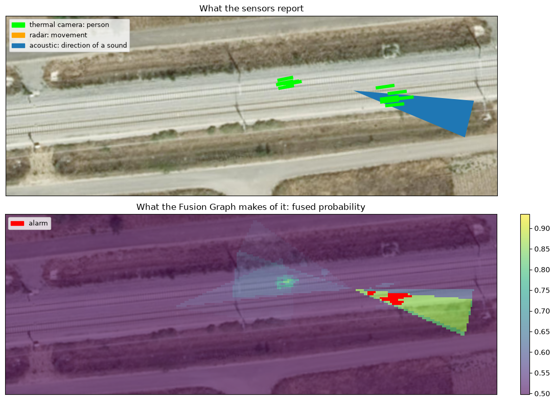
Satellite imagery: Esri, i-cubed, USDA, USGS, AEX, GeoEye, Getmapping, Aerogrid, IGN, IGP, UPR-EGP, and the GIS User Community.
Tip
Experiment with it: drop a sensor from BayesianFusion, or change a decay rate or the threshold,
and see how the alarm changes. That is exactly how the parameters were tuned in the trial.
References#
Project: MOBILIZE, funded by the Austrian Mobility of the Future programme.
Publications:
M. Hubner, K. Wohlleben, M. Litzenberger, S. Veigl, A. Opitz, S. Grebien, and M.-T. Dvorak, “A Bayesian approach – data fusion for robust detection of vandalism and trespassing related events in the context of railway security,” 27th International Conference on Information Fusion (FUSION), 2024.
M. Hubner, K. Wohlleben, M. Litzenberger, S. Veigl, A. Opitz, S. Grebien, F. Graf, A. Haderer, S. Rechbauer, and S. Poltschak, “Robust detection of critical events in the context of railway security based on multimodal sensor data fusion,” Sensors, vol. 24, no. 13, 2024.
M. Hubner, J. Nausner, and K. Wohlleben, “Advanced sensor fusion for railway security – a hierarchical graph-based approach,” Sensor Data Fusion: Trends, Solutions, Applications (SDF), 2024.